- Here is the python script for my ANN model build from scratch with full NumPy style documentations and comments: [Link].
- Column 1 indicates the total population of the polygon area in which the Starbucks store is situated.
- Column 2 records the total number of colleges within the one-mile buffer zone around the store.
- Column 3 reflects the median monthly household income of the polygon area where the store is located.
- Column 4 lists the total number of shopping malls within the one-mile buffer zone of the store.
- Column 5 shows the total revenues for each Starbucks store in 2016, comprising the aggregate of monthly incomes for that year.
- When determining the ideal location for a new Starbucks shop, we primarily considered the store's yearly revenue from the previous year. However, this data did not account for fixed and operating costs, which are crucial in real-world scenarios. For example, while a Starbucks in Beverly Hills, Los Angeles, might predict high revenues, it may not be a viable location due to potentially high rent and operating costs.
- The U.S. Census Bureau's polygon area data shows significant size variations based on location. Larger polygons might naturally encompass a larger population. Therefore, directly recording the population of a polygon area where a Starbucks store is located, without adjusting for the polygon's size, could introduce bias.
- We did not consider the impact of over-competition when deciding to open new Starbucks locations. For instance, despite high population density and median income suggesting that Beverly Hills, Los Angeles, could be an ideal spot for new stores, the area might already be saturated with Starbucks outlets, making it less advantageous to open another store there.
- Our mixed-effects model assumed a linear relationship between the yearly revenue of Starbucks stores and our four regressors. However, this relationship could be non-linear, which the current model does not account for.
- Bates, D.; Maechler, M.; Bolker, B.; Walker, S. (2015). "Fitting Linear Mixed-Effects Models Using lme4". Journal of Statistical Software. 67 (1). doi:10.18637/jss.v067.i01.
- De Myttenaere, A., Golden, B., Le Grand, B., & Rossi, F. (2016). Mean Absolute Percentage Error for regression models. Neurocomputing.
- Gurney, Kevin (1997). An introduction to neural networks. UCL Press. ISBN 978-1-85728-673-1. OCLC 37875698.
- Kruse, Rudolf; Borgelt, Christian; Klawonn, F.; Moewes, Christian; Steinbrecher, Matthias; Held, Pascal (2013). Computational intelligence : a methodological introduction. Springer. ISBN 978-1-4471-5012-1. OCLC 837524179.
- Lawrence, Jeanette (1994). Introduction to neural networks : design, theory and applications. California Scientific Software. ISBN 978-1-883157-00-5. OCLC 32179420.
- McLean, Robert A.; Sanders, William L.; Stroup, Walter W. (1991). "A Unified Approach to Mixed Linear Models". The American Statistician. American Statistical Association. 45 (1): 54–64. doi:10.2307/2685241. JSTOR 2685241.
Executive Summary
This project report presents an in-depth analysis of Starbucks stores across ten major U.S. cities, using a blend of non-public data from UCLA's AtoZdatabases and public data from the U.S. Census Bureau. By mapping Starbucks locations in relation to factors like population density, proximity to colleges and shopping centers, and area income levels, the study visually and quantitatively assesses the influence of these factors on store revenues. Significant findings include a clear tendency for stores to cluster near areas with higher population densities, educational institutions, and wealthier households. A novel approach was taken to merge and analyze these data sets, creating a linear mixed-effects model to understand the revenue implications at both city and national levels. The model's predictive accuracy is notable, with a MAPE of 8.17% and an RMSE of 55734.78, suggesting a reliable method for forecasting revenues of existing and potential Starbucks locations. Additionally, the study transforms revenue prediction into a classification problem, using a multi-hidden-layer Artificial Neural Network (ANN) built only from basic Python libraries. This model comparison indicated that the best performing model had two layers, with varying nodes, minimizing overfitting and providing the most accurate revenue classification with 0.97 test accuracy. This comprehensive analysis offers Starbucks valuable insights into location strategy and potential revenue, aiding in the decision-making process for store expansion.
Data and Exploratory Data Analysis
The Starbucks vector datasets comprise both non-public data from AtoZdatabases at the UCLA Anderson School of Management, detailing monthly revenues and locations for approximately 1,200 Starbucks stores in ten major U.S. cities, and public data from the U.S. Census Bureau. This public data includes information about U.S. population density, the locations of colleges and shopping centers, and income distribution in each polygon area across the USA.
From the following four QGIS graphical maps, we observe that Starbucks shops tend to be clustered near shopping centers, colleges, and areas with high-income households and large population densities:
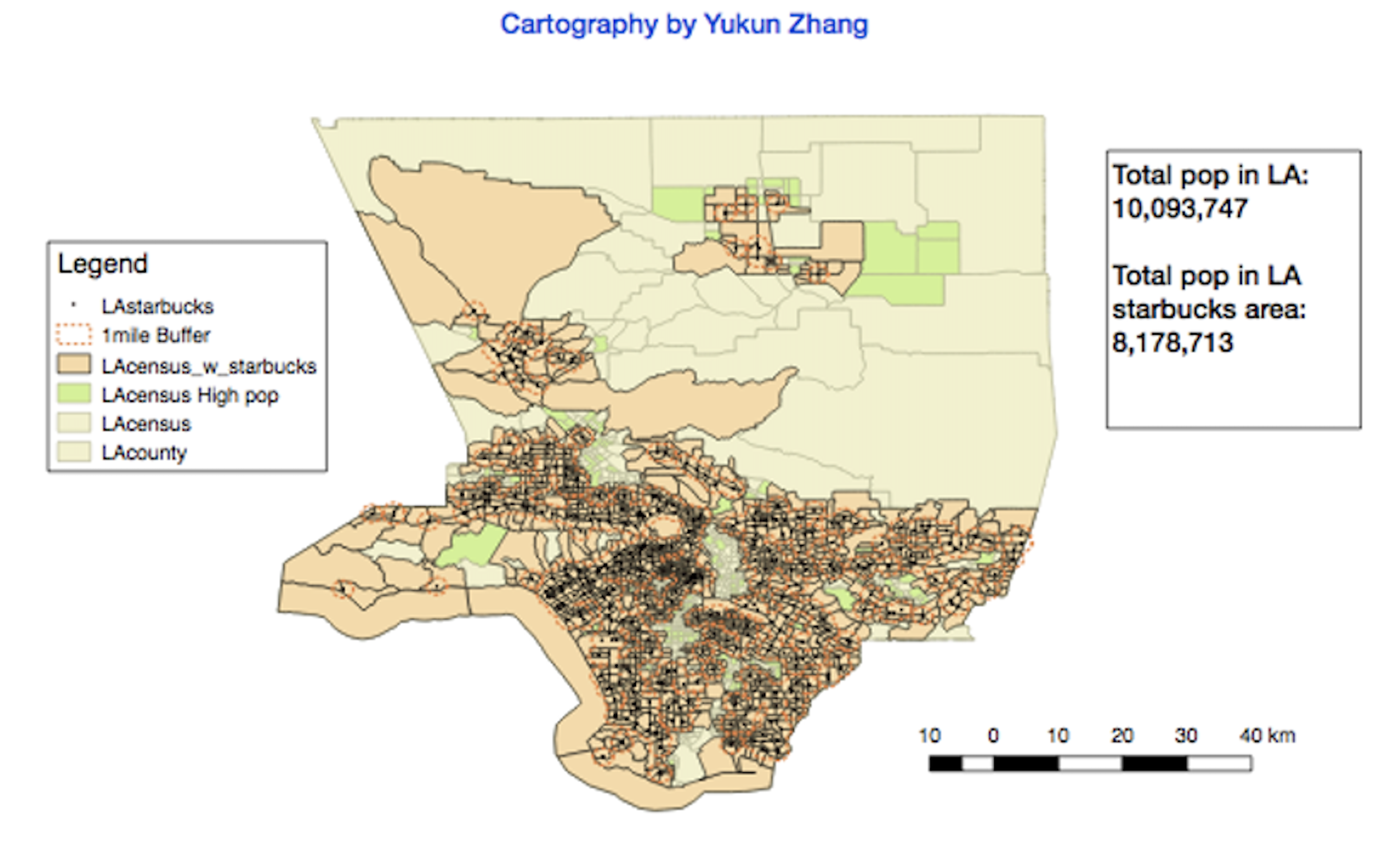
In the above figure, most of the orange areas intersecting our one-mile buffer zones near Starbucks locations have large populations, typically exceeding 5,000 people. The green polygons represent areas with populations over 5,000 that do not intersect with our one-mile buffer zones. Thus, it may be sensible to consider opening a Starbucks shop in these green areas to effectively capitalize on their large population resources for increased revenue.
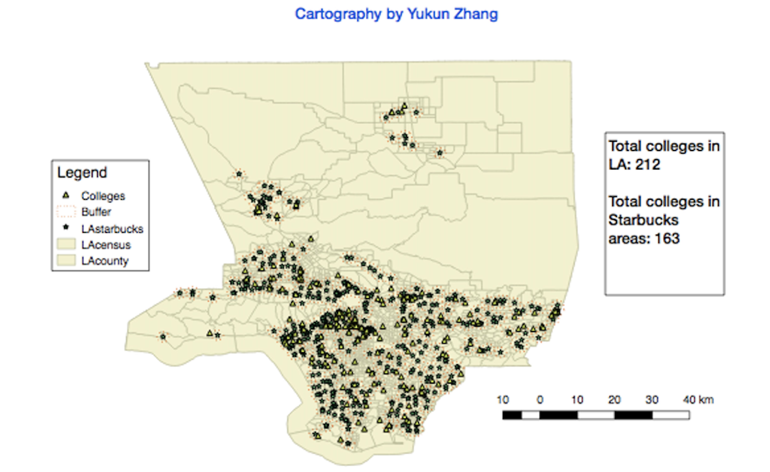
For the above mapping, each small yellow triangle represents a university. Almost all of these are situated very close to the one-mile buffer zones near Starbucks.
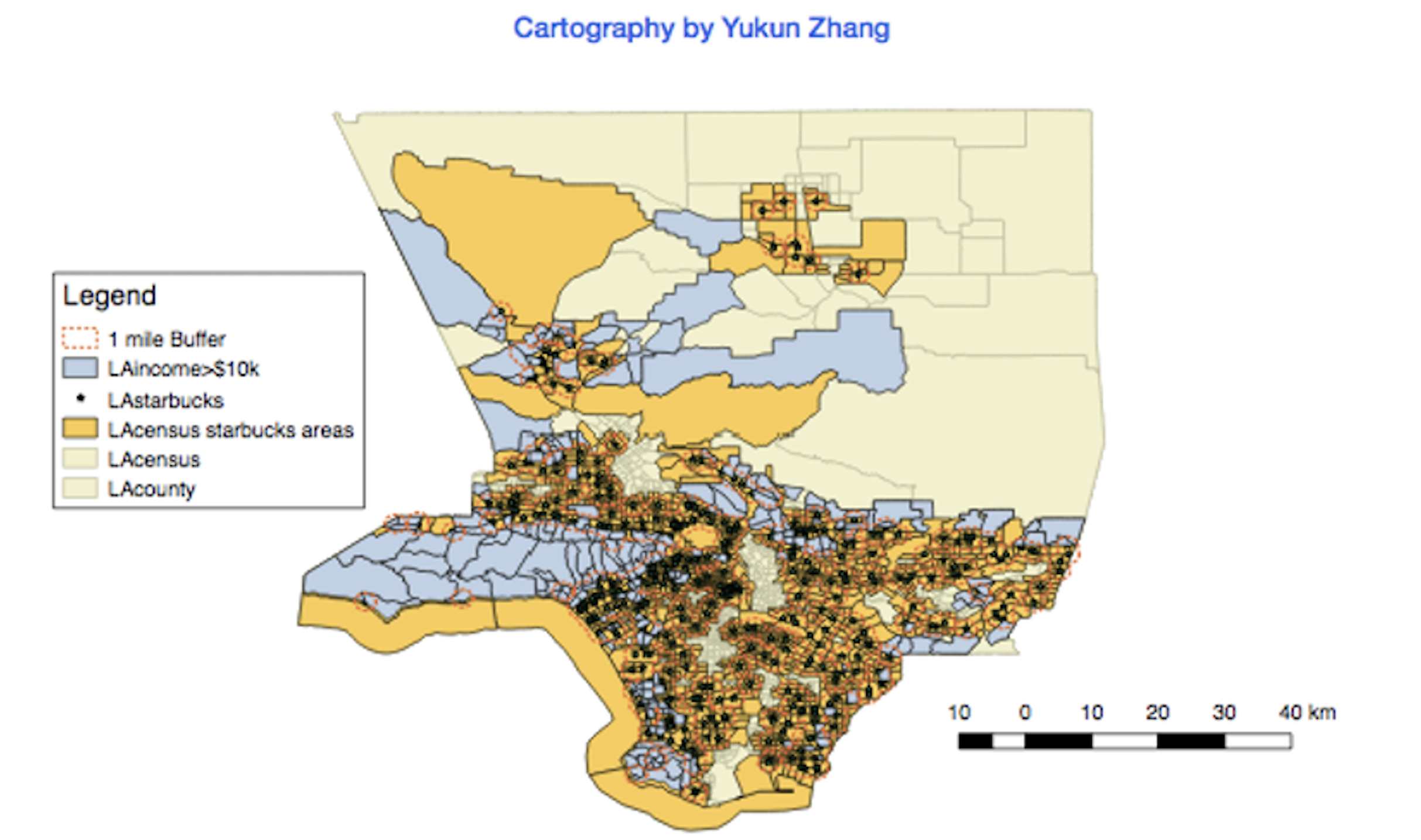
From the above plot, the light blue regions indicate high-income areas where the median household monthly income exceeds $10,000. Many of these blue areas intersect with our one-mile buffer zones around Starbucks.
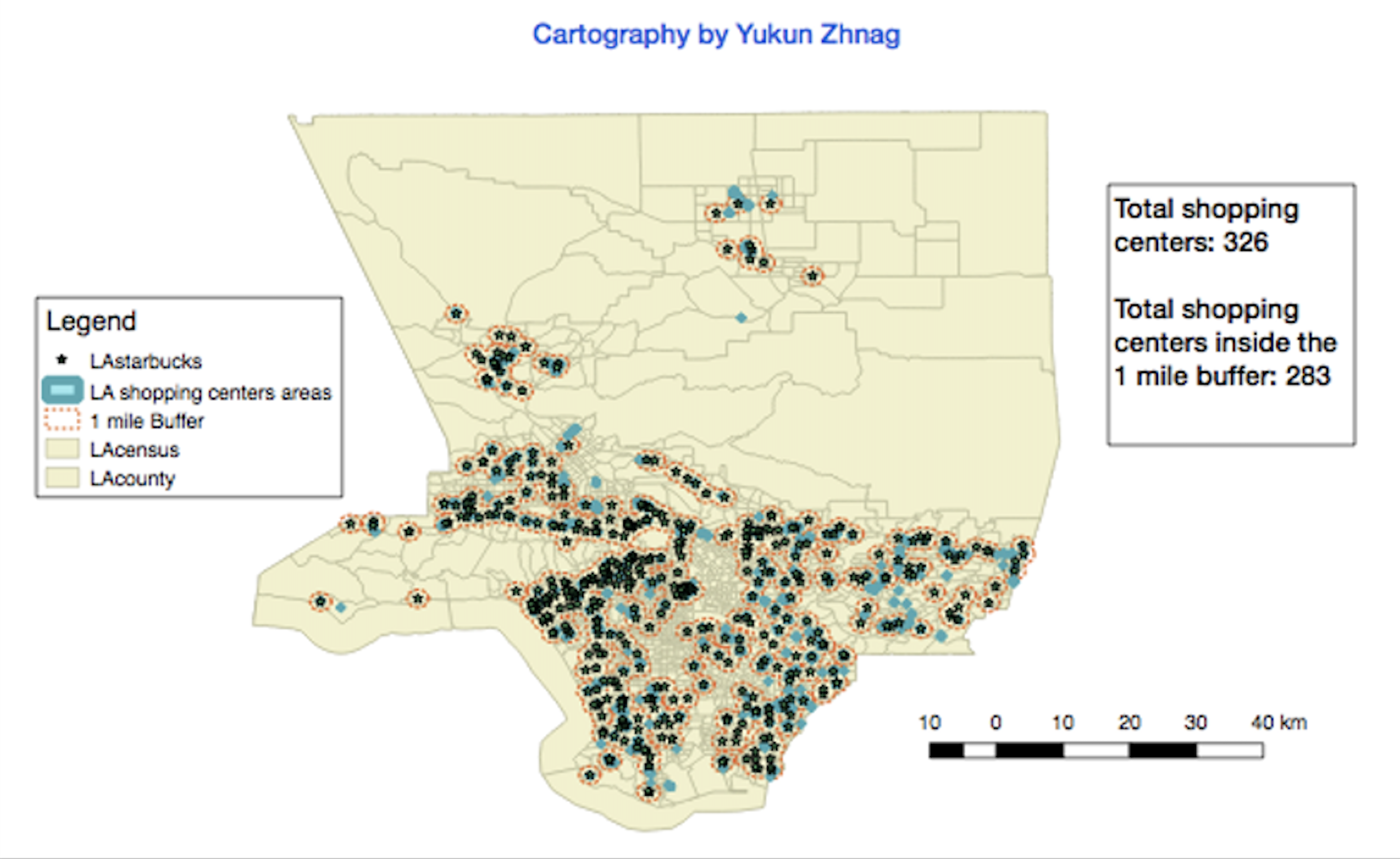
For the last graph above, each small blue dot represents a large shopping center, with nearly all of them located in close proximity to the one-mile buffer zones around Starbucks.
Linear Mixed-effects Modeling
Based on these graphical findings, we aim to further investigate the quantitative impact of the previously mentioned four factors on the annual revenues of Starbucks shops in Los Angeles. Additionally, we are interested in exploring the association between these factors and the annual revenue of Starbucks stores across the entire USA.
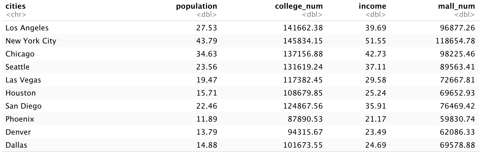
To initiate this analysis, I merged the vector datasets and created five additional columns for each Starbucks store, addressing our research questions. Each row in the dataset represents an individual Starbucks store located in one of ten major U.S. cities: Los Angeles, New York City, Chicago, Seattle, Las Vegas, Houston, San Diego, Phoenix, Denver, and Dallas.
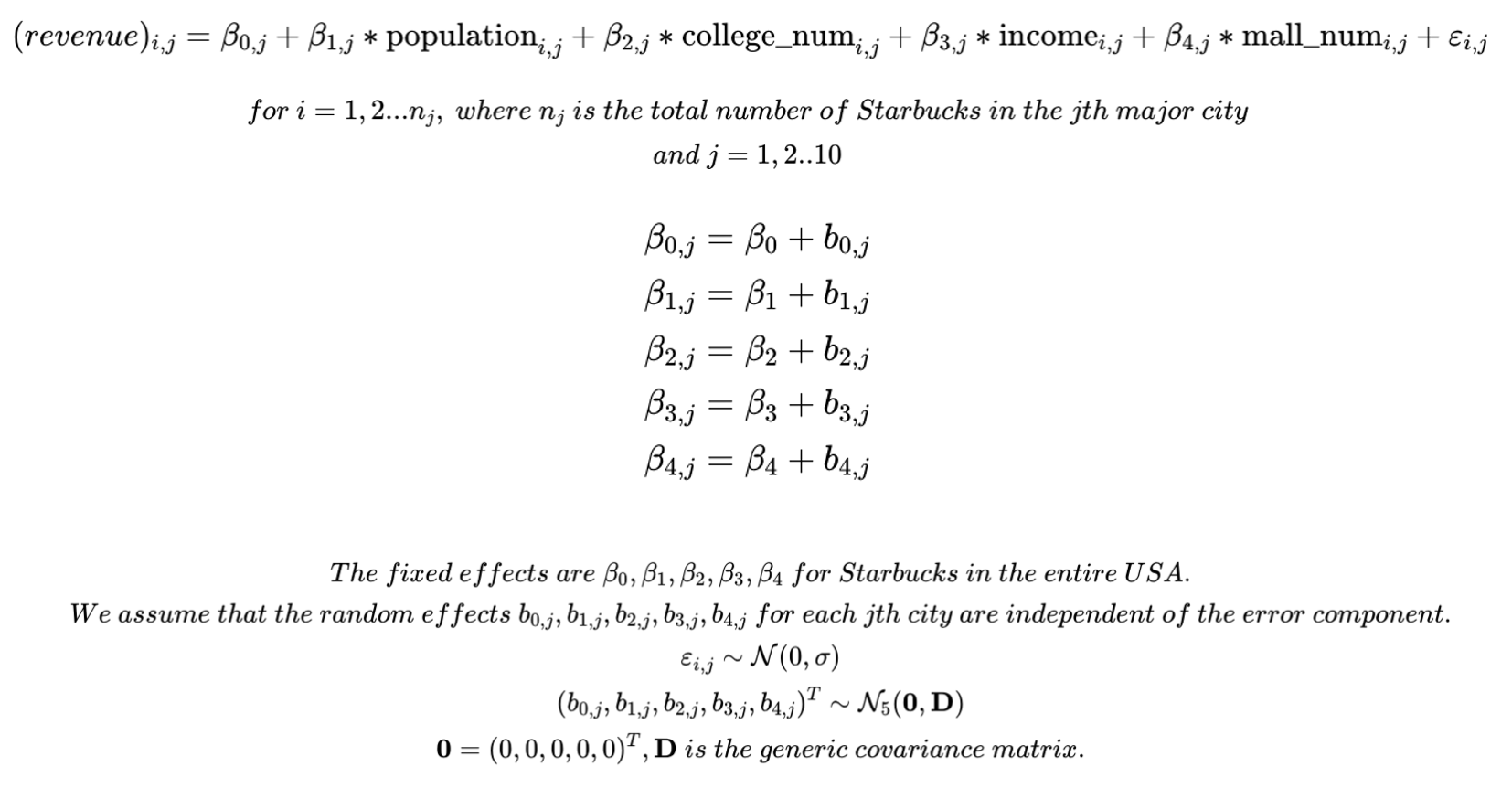
To make inferences about Starbucks across the entire USA using samples from only ten major U.S. cities, we designed our modeling process using linear mixed-effects models. We assume that each Starbucks in these major cities has its own intercept, and there is an overall fixed intercept for all Starbucks in the USA. The model is structured as follows:
We executed the model across the city column using the lme4 package in R. This process yielded significant results with an alpha value of 0.05 for all four Beta regressors (excluding the intercept), which represent the fixed effects on Starbucks' yearly revenue across the USA. The corresponding p-values are 0.014277, 0.000898, 0.036831, and 0.009476, with associated estimates of 21.68, 120213.15, 33.74, and 75745.89, respectively. By summing the fixed and random effects for each city, we calculated the respective coefficients, as presented in the table below:
The predictive Mean Absolute Percentage Error (MAPE) is 8.17%, and the Root Mean Square Error (RMSE) is 55,734.78, indicating the model's predictive accuracy. Based on our results, we can quantify the fixed and random effects of our four regressors on Starbucks' yearly revenue and make informed predictions about the potential yearly revenue of new Starbucks stores in these 10 cities. Moreover, even with the current data, we can make some predictions about the yearly revenue of any prospective Starbucks store in any location in the USA, relying solely on our fixed effects analysis.
ANN Modeling
For Starbucks, a more realistic scenario involves opening hundreds of new stores simultaneously, making it crucial for the upper management team to have a broad understanding of the potential revenue scale. Therefore, I transformed the revenue prediction issue into a classification problem. Initially, I categorized Starbucks' yearly revenue as 'High' for store revenues exceeding $1,000K, 'Medium' for revenues between $500K and $1,000K, and 'Low' for revenues below $500K. Following this categorization, I created a new column named 'revenue_scale' in the dataset. This column uses the total revenue figures to label each store with 'High' as 2, 'Medium' as 1, and 'Low' as 0.
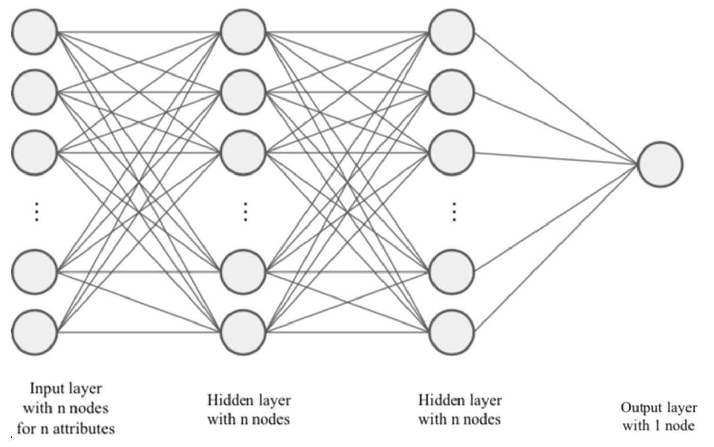
To tackle the multi-class classification problem, I developed the following multi-hidden-layer Artificial Neural Network (ANN) from scratch, utilizing only the basic NumPy and SciPy libraries in Python. This ANN incorporates a Softmax negative log-likelihood loss function, L2 regularization, and Stochastic Gradient Descent (SGD) optimization methods.
Based on an 80:20 split for training and testing of the normalized datasets with fixed seeds, I evaluated the performance of various ANN models, each differing in the number of hidden layers and nodes. The table below summarizes their performances, assessed using accuracy metrics:
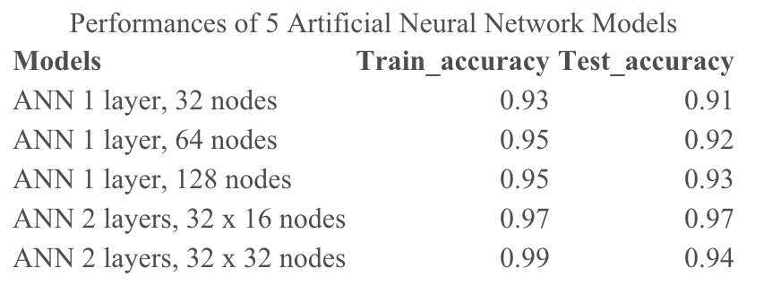
The results reveal that the most complex ANN models, which have 2 layers with 32 nodes in each layer, exhibit overfitting issues, as evidenced by a high training score of 0.99 but a lower test score of 0.94. The most effective model for our classification prediction is the ANN with 2 layers, comprising 32 nodes in the first layer and 16 nodes in the second layer. This model achieved the best test accuracy, which is 0.97.